In this example we will learn how to:

• Implement the rating system for DCs using an extension.
• Manage cash flow accounting in the supply chain.
• Create a delivery system using the Milk Runs and Fleets tables to provide the best possible service level.
• Define auto-adjusting inventory policy to prevent uncertainty of demand.
• Decrease the impact of the stochastic input data on the statistics using the Variation experiment.

Stochastically defined data:

• Customer’s demand.
• Processing time.
• Couriers speed.

Customers are expected to receive the product within a day after they buy it.

The advantage of anyLogistix is the ability to extend any object using AnyLogic simulation software built-in as an extension editor.

In this example, we are using the Online Shop extension, which contains two extended standard objects: DC and customer. Each of the DCs in this scenario has an additional rating variable. Each time a customer receives a shipment the rating for the delivery is generated. If the lead time is higher than expected, then the negative rating is set for this delivery with an 80% probability, otherwise no rating will be assigned. If the expected lead time was not exceeded, then a positive rating is generated with a 30% probability. The average value of the known ratings is set by the customers, receiving products from the DC, forms its rating.

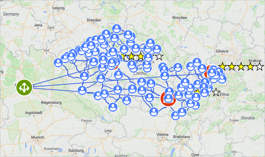
Visually on the map, we can see the rating of the DCs as the number of glowing stars.

The distribution network in this example contains Cash Account and Payment Terms to manage financial flows. The key parameters are:

• Initial cash = $100 000.
• Days payable outstanding (DPO) = 15 days.
• Days sales outstanding (DSO) = 30 days.
• When the distributor purchases product from the supplier the down payment ratio is 20%.
• When customers order smartphones from the distributor the down payment ratio is 30%.

Delivery to the customers is made by the couriers, which are assigned to the DCs. The number of vehicles assigned to the DCs is defined in the Fleet table. The values are 20, 10, and 6 for DC Prague,DC Brno, and DC Ostrava respectively.

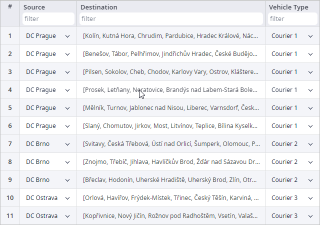
Since we have a limited amount of fleet, we need to optimize product delivery to the customers. To do that we defined the milk run routes to deliver products to several customers per trip. These routes are defined in the Milk Runs table.

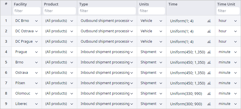
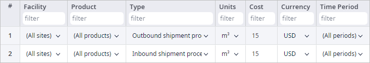
To define a more precise product delivery process we defined the time and expenses required to prepare vehicles and shipments for delivery, loading, and unloading products, etc. This data is defined in the Processing Time and Processing Cost tables.

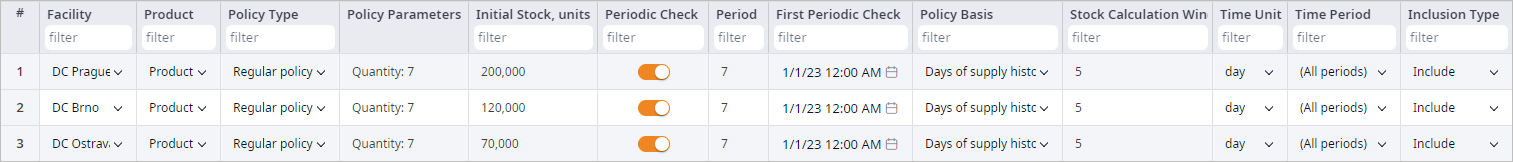
Inventory for the DCs is defined using Days of supply historic. It allows us to not define the actual values of selected inventory policies, but specify the number of days for which the average demand will be calculated, and the number of days for which this DC will be ordering the product, considering the future demand.

Run the Simulation experiment and analyze statistics.

Run the Variation experiment to get the aggregated statistics without stochastic impact on the results.

The Online shop extension also provides custom statistics:

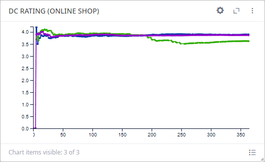
• DC Rating — data on DCs rating within the supply chain.
• Positive Feedback — data on the amount of positive feedback a DC received.
• Negative Feedback — data on the amount of negative feedback a DC received.
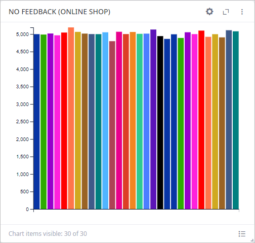
• No Feedback — data on the number of customers that left no feedback.

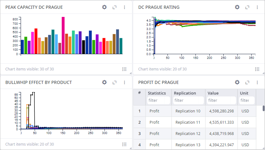
On the first chart of the Service level tab we can see the DC Rating statistics. Rating value for each DC consolidates at 4 stars.

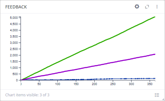
The Feedback chart shows aggregated feedback statistics. As we can see, the majority of orders were not rated, and positive rates prevailed.

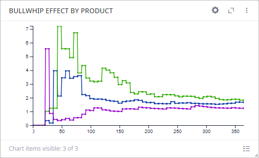
Also, on the Bullwhip Effect tab we can see the chart that shows statistics on product demand variability amplification during the simulation: from the point of actual (final) product demand to the point of origin. DC Brno was the one most affected by the bullwhip effect.

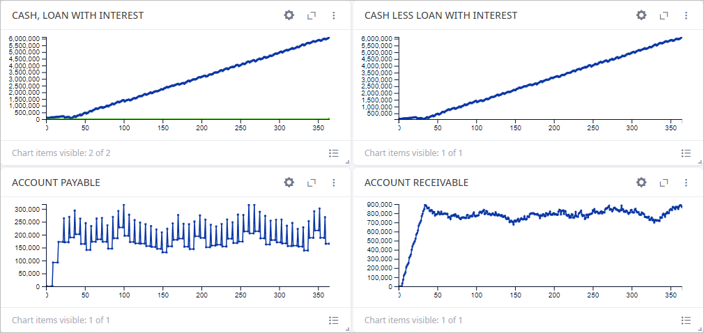
In the Cash to Serve tab, we can see statistics on financial flows throughout the supply chain cash account.

Now let us run the Variation experiment.

The experiment will repeatedly run a Simulation experiment, producing statistically significant results, collecting statistical data, and providing the result in a table.

Variation experiment allows us to estimate the effect of stochastic parameters on the supply chain.

As we can see, the max capacity of the DC Prague storage is fluctuating from 253 to 851 m³, which is more than 3 times the difference.

Feedback also differs from iteration to iteration.

These differences between the runs explain why we should analyze aggregated variation results instead of looking at just one simulation run when using stochastic data as input.

anyLogistix extensions to create a powerful and flexible simulation model. They are built using AnyLogic extension editor and help to simulate your unique processes, which cannot be defined by the default options.

How can we improve this article?

Send