

In this example, we will learn how to select a defined number of facilities considering facility expenses and costs of Inbound shipment processing and Outbound shipment processing.
This scenario was created by converting the results of the GFA scenario to an NO scenario and adding extra details. The scenario is a part of the sequence of 4 example models that illustrate the different stages of supply chain analysis:
- GFA US Distribution Network — a scenario for finding location areas of warehouses.
- NO US Distribution Network — a scenario for selecting facilities from the suggested list of distribution centers and Ports. This is the scenario we will investigate now.
- SIM Distribution Network Analysis — scenario that is based on the result of the optimization. This result has been converted to the SIM scenario to analyze the suggested network in more detail.
- SIM Budget Comparison — a scenario for analyzing the impact of unstable demand on the service level of the supply chain.
All the input data can be found in the previous example of this sequence.
In the previous example — GFA US Distribution Network we used the GFA experiment to find the following areas for regional distribution centers: North (Oregon), West (Nevada), South (Texas), and East (Virginia). We can make this a new NO scenario by converting the obtained results to the NO scenario.
We decided to use only 3 regions from the GFA experiment results. For every region, we defined several possible locations of distribution centers.
Also, we added supplier for the products located in Rio de Janeiro, Brazil. To transfer products from supplier to distribution centers we will use Ports, located in the US, and distributed along the coast. We will consider group of ports in this scenario. From the ports the product will be shipped to the distribution centers, and then to the customers.
For every distribution center we defined Initial cost and Other costs, to specify the expenses on opening and maintaining warehouses. All these costs are defined in the Facility Expenses table.
Also, for every facility, we defined Inbound shipment processing and Outbound shipment processing. These costs define the expenses on transshipping products in the facility (loading/unloading from the vehicle). See the Processing Cost table for more details.
All these costs will be used in calculation of the objective function to find the best possible solution considering the following restrictions:
- We can open only one distribution centers in the West, South, and East regions.
- We can use only one port for transshipment.
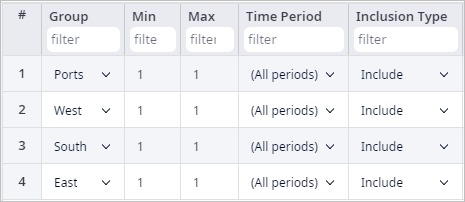
These restrictions can be defined in the Assets Constraints table.
Find the most suitable warehouse locations in every area, and choose a port, which will be a transshipment base between the supplier in Brazil and the regional distribution centers.
The result offers 10 the most profitable warehouse locations. The best choice is to open distribution centers in Lynchburg, Reno, Austin, and use the Port of New Orleans for transshipment.
The Iterations panel shows the result of the experiment with all the possible combinations sorted per the Profit KPI metric.
The top iteration card is the best one.
The data on other details is shown in the corresponding tables:
The next step is SIM Distribution Network Analysis, where we convert the results of the NO experiment to the SIM scenario and perform a simulation run to analyze the detailed statistics.
-
How can we improve this article?
-