In this example, we will learn how to analyze the data collected from the simulation experiment. We will also learn how to define operating hours for the facility within defined days, when received orders can be shipped to the order destination.

The actual scenario data can differ from this description if you are using the PLE version.

This is the continuation of the example NO Global Network Optimization. All the input data is defined in the previous example description.

We used the NO experiment to find the most suitable warehouse locations in every area:

• North America (Dallas)
• South America (Sao Paulo and Buenos Aires)
• Europe (Brussels)
• Russia (Moscow)
• India (Chandrapur)
• China (Nanchang)

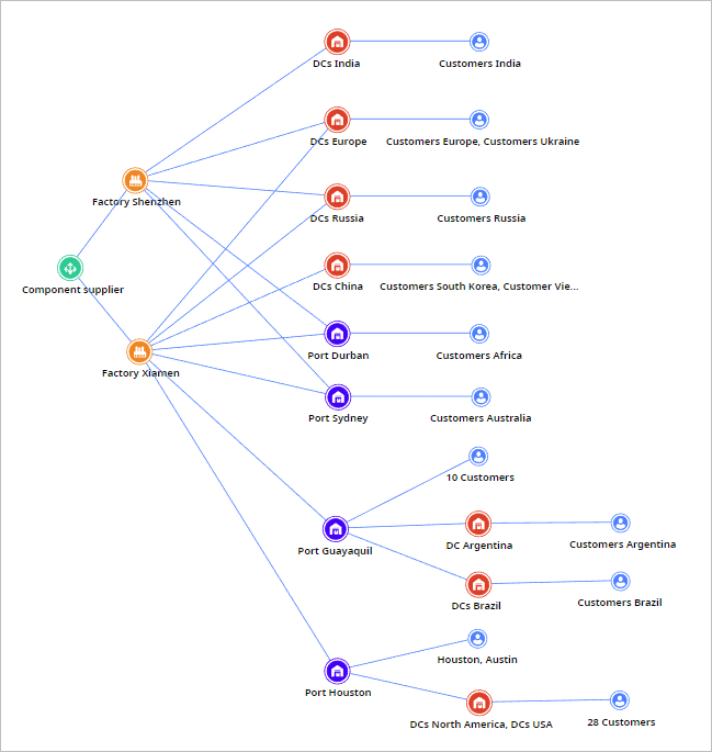
This scenario was made by converting the results of the Network optimization experiment from the previous step of the sequence. We can observe the structure of the supply chain by opening the Structure view of the scenario. Here we can see two factories supplied by the Component’s supplier. Factories produce finished products and ship them to 4 DCs (by air and roads), and to 4 Ports (by sea). Ports deliver the received products to the remaining DCs, or directly to the customers. Finally, All DCs serve defined customers group.

In addition, we can set operating hours: days of week and time when shipping can be initiated to deliver products from the specified source to the specified destination. If the order is received out of the operating hours, it will be postponed until the next working period of time. This schedule is defined in the Shipping table.

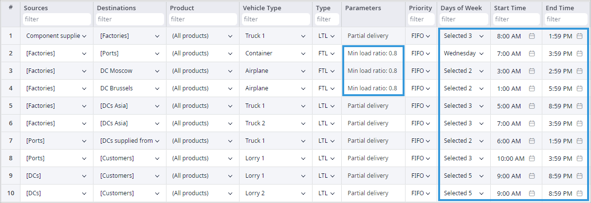
In the Shipping table we defined type of shipping policies (FTL and LTL). The difference between these two types is that for the FTL we can define the Min load ratio. This parameter shows the minimum fraction of truck capacity that should be filled to allow this vehicle to set off. If the received order does not have enough products, the vehicle will wait for the next order for the same destination to later deliver them all. In our case, we defined the FTL policy for the Airplane and Container deliveries since it would be a waste of money to send a half-empty vehicle.

As your manufacturing plans have to meet the requirements of your supply chain including demand, shipping terms, downstream inventory policies, etc., you need to calculate the ROI of your network change decisions.

A simulation experiment is used to model the delivery of the actual product on the GIS map with detailed statistics, which show the data collected on different types of facilities involved in the supply chain scenario during the experiment.

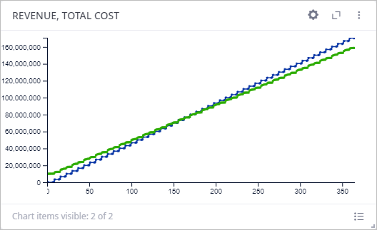
On the first tab of the dashboard we can see the data on revenue, total cost, which show that the supply chain required about $10 000 000 as an initial investment. Supply chain started to gain revenue during the simulation period, which led to the break-even point on the 176th day of simulation.

You may continue to observe statistics, collected by the Simulation experiment on the dashboard:

• Service Level — statistics on service level collected by the number of available products and by expected lead time.
• Lead Time — statistics on time spent on delivery products to the customers.
• Available Inventory — here collected data of products located in DCs storages (On-hand Inventory), and the actual number of products available to delivery.
• Fulfillment — statistics on received and fulfilled product orders from customers and DCs.
• Etc.

How can we improve this article?

Send