

In the previous phase we analyzed the locations offered by the GFA experiment, defined alternative distribution centers locations considering infrastructure, specified product supplier, and set assets constraints.
In this phase we will add financial information which will mostly refer to the expenses the supply chain incurs. We will specify the cost of opening a distribution center for every potential location. The cost will obviously differ from city to city due to numerous factors. Alongside this, we will specify the cost of processing the outgoing shipments for every potential location. We will also set the cost of obtaining a product as well the selling price. The Network Optimization experiment will consider the new data which will make the results it offers more accurate.
Let us start with specifying the cost of obtaining one item of PS4 console and its selling price.
Specify the self-value and the selling price of a PS4
- Click the tile with your scenario name to switch to the supply chain mode (the dashboard will contain tables with scenario data).
- Navigate to the Products table and specify 399 in the Selling Price column cell. This is the retail price of the PS4 console for all customers.
- Now specify 381 in the Cost column cell. This is the cost of obtaining one PS4 console.
As you might have noticed, the difference between the obtaining cost and the selling price of a PS4 unit constitutes $18 only. This is due to the fact that Sony is making money not on selling its console but on selling software (games) for its console. Let us run the Network Optimization experiment to see how these changes affect the result we will receive.
Run the Network optimization experiment
- Navigate to the Experiments section, click the Network optimization tile, then run the experiment by clicking
 Run on the experiment's tile.
The results will be available in the Result 2 item.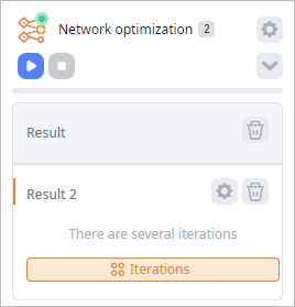
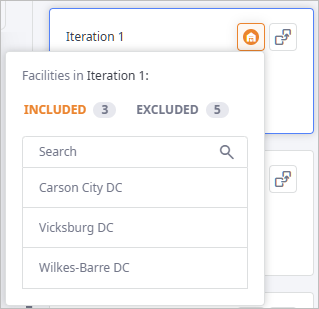
- Analyze the received data in the Iterations panel.
-
The top iteration card still offers the best solution, and if we click the
 Facilities in iteration # icon, we will see the same set of distribution centers.
-
Now look at the metrics in the KPI ribbon of the Result 2 Dashboard below the map.
The KPI metrics added to the ribbon are automatically compared to the KPI metrics of the previous result of this experiment, which is the Result item.
We can see that the value of the Profit metric is now positive:

-
The top iteration card still offers the best solution, and if we click the
Now we will specify the Initial cost for all potential distribution centers locations. This will inevitably affect the Profit value, but we are mostly interested in the locations the experiment will offer us considering the additional expenses.
Specify Initial cost values
- Click the tile with your scenario name to switch to the supply chain mode.
- Open the Facility Expenses table and click Add to create a new record.
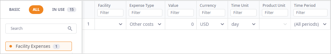
- Double-click the Facility column cell and select Carson City DC from the drop-down list.
- Double-click the Expense Type column cell and select Initial cost from the drop-down list.
- Click the Value column cell and set 12,092,000 as the cost of opening a facility in Carson City.
The record should look like this: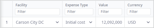
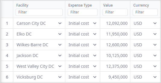
- In the same way specify the cost of opening a facility for each distribution center location that is not marked as Excluded,
as shown on the screenshot below.
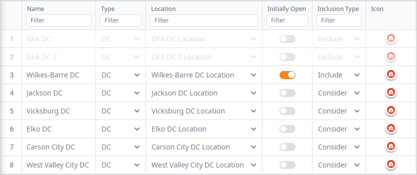
- Navigate to the Distribution Centers table and change the Initially Open
state for all the alternative distribution centers as shown on the screenshot below. If we do not toggle the state, the
experiment will consider the facilities initially open, as a result no expenses will be incurred.
When done, proceed to specify the cost of processing outgoing shipments.
Specify cost of processing outgoing shipments
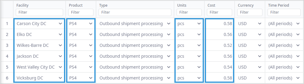
- Open the Processing cost table and create six table records by clicking Add.
- Now specify the product and the cost of processing one console unit in the outgoing shipments for every distribution center, as shown on the screenshot below.
Now let us go back to the Network Optimization experiment and run it again.
Run the experiment and compare results
-
Navigate to the Experiments section, click the Network optimization tile, then run the experiment by clicking
Run on the experiment's tile.
The results will be available in the Result 3 item. -
Analyze the received data in the Iterations panel:
-
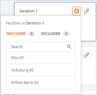
Click the Facilities in iteration # icon of the top iteration card.
As you can see, the best distribution centers locations in terms of the specified costs are: Elko DC, Vicksburg DC, Wilkes-Barre DC.
-
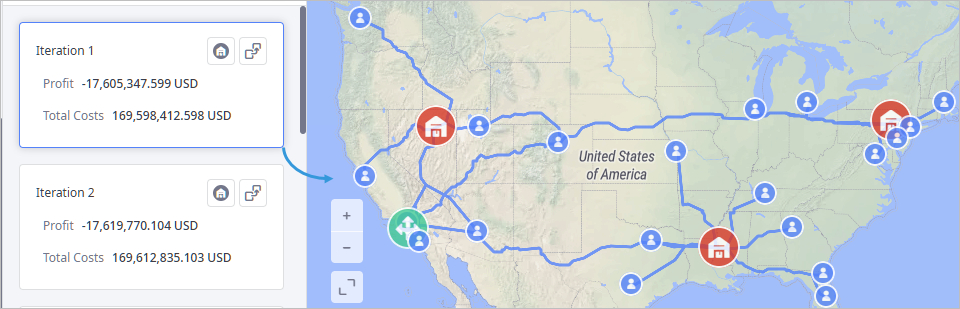
Now check the metrics in the KPI ribbon of the Result 3 Dashboard.
As expected, the costs increased and the profit decreased.

-
Click the
-
The top iteration card in the Iterations panel of the Result 3
item is selected by default, so you may observe it on the map.
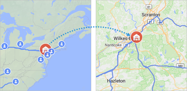
You may enable visualization of sourcing paths and zoom in to each offered distribution center location to examine its paths to the customers it services, as we did on the example of Wilkes-Barre DC below.
We have found the best supply chain configuration using analytical optimization methods. The received result considers:
- Suggested warehouse locations
- Actual available roads
- Transportation costs
- Site opening costs
- Processing costs
Now we will convert this result to a scenario to modify it later and use it in the Simulation experiment, for example.
Convert Network Optimization experiment results to a scenario
-
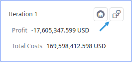
Click the
 Convert to a new scenario
icon in the top iteration card of the Result 3 item.
The Convert Result dialog box wil open.
Convert to a new scenario
icon in the top iteration card of the Result 3 item.
The Convert Result dialog box wil open.
- If required, change the Scenario name.
-
Define the type of scenario, to which the result must be converted by clicking the
 Network optimization scenario type label.
- Finally, click Convert to convert the result.
Now, that you have converted the experiment result to the NO scenario, you can observe the data from the result in the anyLogistix tables. Basically, we have two tables that acquired additional data as compared to the initial scenario without the results of network optimization.
Observe experiment results in tables
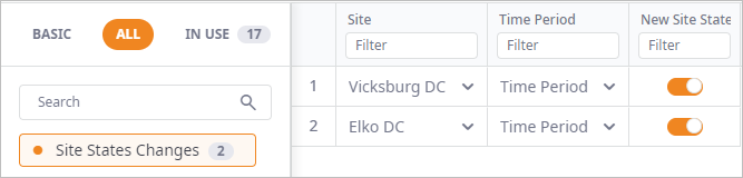
- Navigate to the Site States Changes table of the newly created scenario.
This table contains the best distribution centers locations additionally to the included Wilkes-Barre.
- Now move to the Product Flows, which now contains significantly more records.
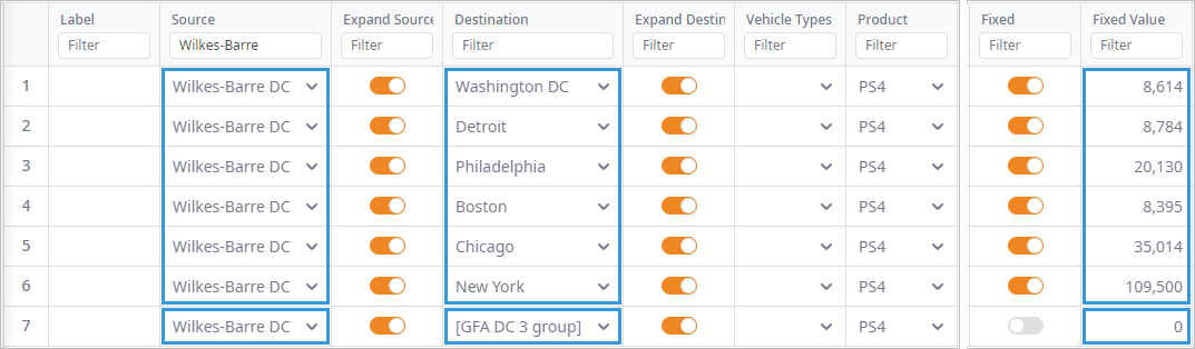
Filter the data by typing Wilkes-Barre into the empty field below the Source column name.
The table contains the following set of records:- Records 1-6 were generated during the experiment. These are the flows from a particular distribution center to every customer it services.
- Record 7 is the product flow (one of the three flows) that we modified in the first phase. It is
based on the data derived from the Sourcing table on converting GFA scenario to NO scenario.
Experiment considers all records of this table, since they do not contradict each other and complete our supply chain.
- The Fixed Value column shows data on the throughput of each source/group of sources.
We have successfully completed the Network Optimization tutorial.
This new scenario can now be used in the Simulation experiment for further supply chain optimization.
-
How can we improve this article?
-