In this example we will learn how to create procurement schedule of raw materials for a supply chain using shipment scheduling statistics. We will also update this supply chain to make it work on the created schedule. And finally, we will perform a stress-test of the supply chain considering disruptions, and we will assess the reliability of the created schedule.

A clothing manufacturer wants to create a schedule that would show when, how many, and from which suppliers the raw materials should be ordered. This schedule will then need to be stress-tested for possible disruptions.

To make this kind of schedule we need to gather and analyze information on available suppliers.

We consider a supply chain in India comprising:

• The factory in Shegaon producing different types of clothing.
• 10 suppliers selling fabric required for clothing production.
• Garment accessories supplier (buttons, zippers, etc.), which are used in most of the clothing.
• The treads supplier.
• 10 distribution centers in India, from which the finished clothing is sent to the customers.
• 100 customers in India.

The finished products are shipped to the customers from the distribution centers by small trucks.

Demand is periodic (first order is placed at a random moment within the 10 days interval) and is proportional to the population of the cities.

• Get a shipping schedule that will show the exact number of products to order from the exact supplier at the exact moment of time.
• Check how reliable the received shipping schedule is, considering possible supply disruptions.

To achieve these two goals, we need to consider two scenarios:

• SIM Procurement Schedule Creation, in which the shipment schedule will be generated.
• SIM Procurement Schedule Stress-Test, in which we will verify and stress-test the generated schedule.

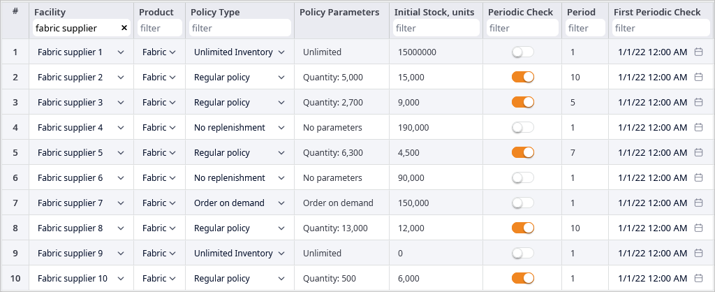
In this scenario, we specify different behavior for suppliers, since each supplier is representing a different production facility. To be able to define the required behavior, we created suppliers with the help of the Factory object type. These objects will have their own inventory policies. Certain Fabric suppliers are using regular policy, and offer different types of fabric in batches which become available once in several days. Other suppliers do not offer certain types anymore and can only sell what is left in their storages. There is also a couple of suppliers that can sell any amount of fabric.

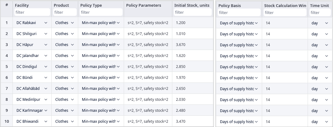
The defined Min-max policy with safety stock for the Shegaon Factory and the DCs is based on the days of supply historic. This method is based on demand forecast and can adjust the amount of product to order depending on the situation. It allows us to define not the actual ordering values, but the number of days for the demand forecast that this policy considers.

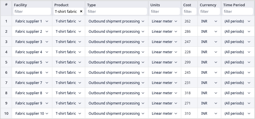
The cost of fabric differs for every supplier. We can specify that with the help of the Outbound shipment processing cost policy from the Processing Cost table.

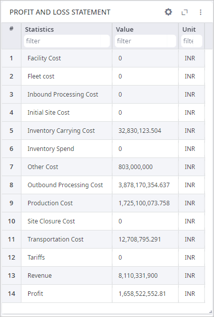
The Outbound shipment processing cost in the Profit and Loss Statement statistics will now represent the costs on raw materials instead of the Inventory Spends, as it is usually done when a supplier is represented by an object of the Supplier type.

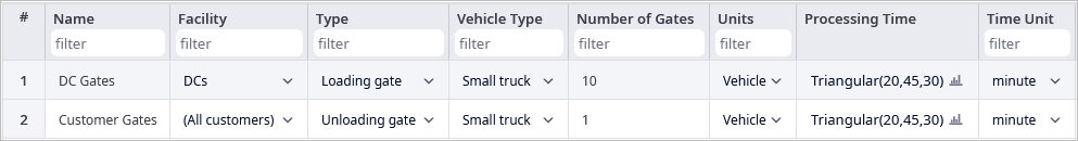
The supplier’s production time is set to 0. There are no bills of materials for it, because the behavior and the fabric costs are already defined. Also, we defined the additional time, spent on loading and unloading products from DCs to customers. This additional time is defined in the Loading and Unloading Gates table which also shows that each DC has 10 Loading gates. That means that 10 vehicles can be loaded simultaneously. The loading times are defined by the triangular distribution. The unloading process on the customer's side requires the same amount of time, but the number of gates is limited to 1.

After running the Simulation experiment, we can observe its results.

On the Profit and Loss Statement tab, we can see the basic statistics on supply chain performance. As we can see, Revenue is greater than Total Cost, and Service level value is almost perfect. Based on that we can roughly conclude that the supply chain works fine. So, we create a real-life shipment schedule with the shipment statistics generated by the simulation model (dates, times, amounts, etc.).

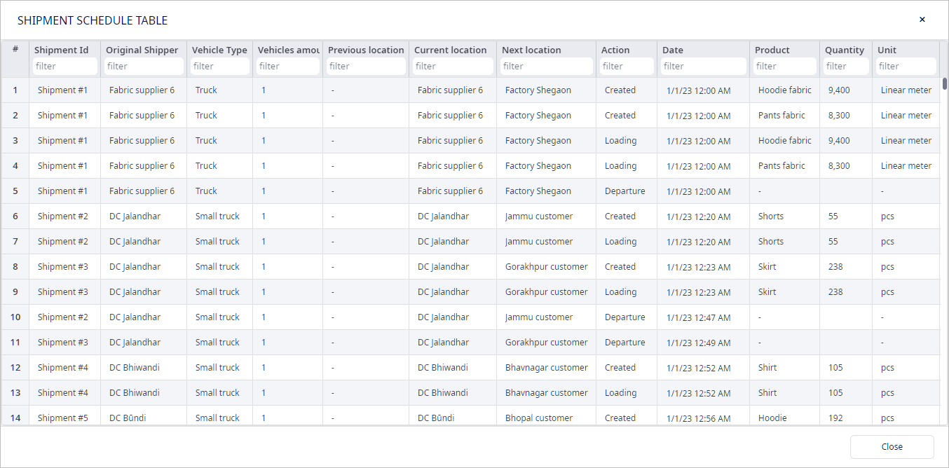
Let us observe the Shipment Schedule Table and the Shipment Table from the Shipment Schedule tab. These tables contain information about all the shipments within the simulation period. The Shipment Table contains data about the financial part of shipments, while the Shipment Schedule Table contains the actual schedule with times required for Loading, Departure, Arrival, and Unloading.

With this, we consider the first goal achieved. Now we can create a shipment plan for our company based on this schedule. However, the schedule itself is not enough. As a company, we need to be ready for disruptions and be able to adapt our plan accordingly. In the second scenario we will stress-test this schedule and develop ways to overcome possible disruptions.

This second scenario contains the converted data from the Shipment Schedule Table from the scenario 1 results in the Push: schedule shipping policy format. This way we introduce the fixed shipment plan into the model.

The Push: schedule policy is defined separately for every Fabric Supplier. The date and time specified in the Policy Parameters are taken from Shipment Schedule Table of the first scenario's results, namely from the Date column's records that refer to the Departure lines of the Action column.

Note that the inventory policy should be set to No replenishment when using the Push: schedule shipping policy, to prevent possible conflicts.

After running the simulation experiment we can check the results. As we can see there is a slight difference in results because of the stochastic way of defining the initial data: Demand, Loading and Unloading times.

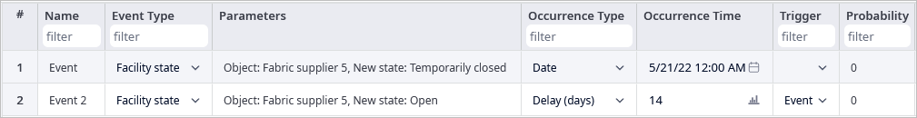
To stress-test this schedule, we can simulate the situation when one of the suppliers stops working for 2 weeks. We can do that by adding 2 events, one to stop the factory and one the other one to open it again after 2 weeks. Events are already added, we only need to change their probability to 1.

Let us run the Simulation experiment to check the impact of events on the supply chain performance.

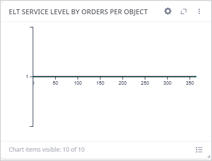
In the Profit and Loss Statement tab of the Simulation results, we can see that the ELT Service level remained 1 for the entire simulation duration even though one of the fabric suppliers stopped its production for 2 weeks. This means that the breakdown happened to the Fabric supplier 5 did not affect the product delivery to the customers.

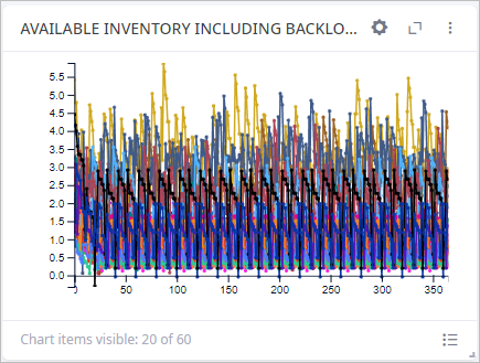
Now we can open to the Available Inventory tab of and observe the Available Inventory Including Backlog per DC chart. It shows the amount of product left in the DCs inventory less the quantity of the processed products for the incomplete orders. As we can see on the chart, the value rarely goes below 0, which proves that the DCs have enough products in storages to fulfill the demand of the customers.

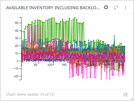
But the breakdown inevitably affected on the factory stock and its performance. On the Available Inventory Including Backlog per Product in Factory Shegaon chart, we can see that the fabric amount significantly decreased at certain points during simulation. That is the consequences of the supplier's breakdown. Several shipments from the schedule were cancelled because of that. But the initial number of raw materials allowed the factory to continue production, and we can see that the pattern of the finished clothes stock did not change much. That is why there is no disruptions on the chart above and in the service level of the customers.

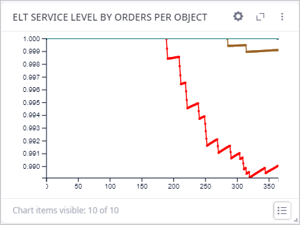
Looks like the supply chain and the created schedule have some room to smooth out the effect of disruption in the early stage of the supply chain. But this room is not infinite. If we increase the supplier recovery time in events by 2 more weeks, and run the simulation again, we will see that not only the available inventory in factory storage decreases significantly, but also the product shortage impacts the customers. We can see that in the ELT Service Level chart.

Using procurement schedule is a very convenient way to maintain product stock of a facility. But it also has its disadvantages, which can have a significant impact on the supply chain performance. To maintain the maximum service level the company should periodically monitor the product stock level as well as the availability of the suppliers.

How can we improve this article?

Send