This example shows the usage of Comparison experiment to analyze a baseline scenario against a what-if scenario. In this example, we compare two possible network configurations — they represent supply chains with same customers and demand but with different sourcing and production.

We consider supply chain of the company selling toasters in the EU countries.

• This company is buying finished products from the supplier located in China.
• The products are shipped from the Port of Hong Kong by the container ship to the Port of Marseilles.
• The containers with product are then transferred to the main warehouse in Marseilles.
• Part of the product are transferring from the main warehouse to the additional warehouses in Düsseldorf and Vienna.
• Part of products that is left in the Marseilles DC and products from the additional warehouses are shipped to the customers.

Customers in this supply chain are retail stores of electronics.

The company is currently thinking about the idea of opening its own factory, in which it is going to produce toasters instead of buying and shipping products from China. The process comprises three steps:

• Find suppliers which will provide raw materials to produce toasters.
• Find a location for the factory, which will be producing components from the raw materials, and assemble the finished products.
• Update the current structure of the supply chain for new source of products (including new capacity of warehouses, new locations for warehouses and different routes for shipment).

Demand is proportional to the population of the cities. It is stochastic with the first occurrence in random time within the defined interval. The order interval is 6 days in average.

Analyze and compare both supply chain structures to decide whether it is better to stick with the existing working system or to start your own production, and completely change the supply chain structure.

Achieving the goal requires a certain succession of actions with these scenarios.

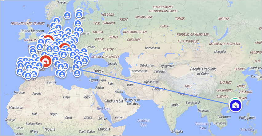
In the baseline scenario the products are delivered from the supplier in China.

After enabling Show connections filter on the map, we can see that the path between the two ports is straight, since it is the route of the ship. For correct calculations the transportation time and the distance were additionally specified for this route. Transportation cost for this path will be calculated using a custom scenario unit (Container). Shipping by this path is only possible once in 14 days.

The Cross Dock policy was chosen for both ports because we don’t have the opportunity to store our product there. The ports are used as the place to transship products from one vehicle type to another.

Export tariffs should be considered for delivering product from one country to another. In case of this scenario the import tariff on toasters on the territory of the European Union constitutes 2,7%. The taxes are defined in the Tariffs table.

Inventory for the DC Marseilles is defined using Days of supply historic feature. It allows us to not define the actual values of the selected inventory policies, but instead specify the number of days this policy is defined for. Since products should be ordered considering delivery from China, we defined Policy Parameters for Min-max policy of DC Marseilles as s = 26, S = 30, safety stock = 6. This means, that if the available inventory drops below the required amount for 26 days, the ordered quantity will equal the inventory quantity required for 30 days, considering safety stock.

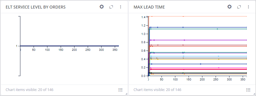
After running the Simulation experiment, we can examine the results. The ELT Service level remains at level 1 during the whole period of simulation, which means that every order from customers was fulfilled within the expected lead time. We can confirm that by looking at the data gathered in the Max Lead Time table that is always less than the expected lead time (which is set to 2 days). The available inventory in every DC is not dropping below 0 which proves that the supply chain operates without issues.

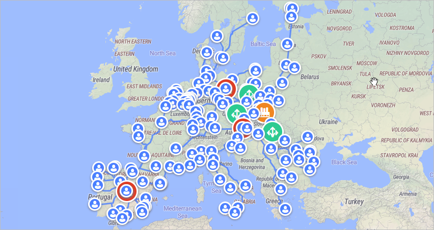
The second scenario contains the supply chain with the company's own production in Poland.

Three new suppliers are located in Poland, Czech Republic, and Hungary. From these new suppliers raw materials and certain components are delivered to the new factory in Krakow, where the metal frames and the bodies are produced, and the assembly of finished products is performed. The production process specifications can be found in the Production and BOM tables. The Production table defines production in this scenario. For example, every 12 seconds the Factory produces 1 new toaster. The Bill of Materials for the toasters is located in the BOM table and contains a list of components and their quantities needed to produce the end product.

Factory can produce Metal frame and Body at the same time and there is no requirement for producing it beforehand. That is why, the Order on demand inventory policy is set for the factory for these products.

Since the expenses on opening new sites have to be considered in results, the state of the sites is set to Initially closed before simulation.

After running Simulation experiment, we can examine the results.

As we can see in the ELT Service Level table, its value remains 1. Because we decided to have the same customers and demand, the Expected Lead Time in this scenario is the same.

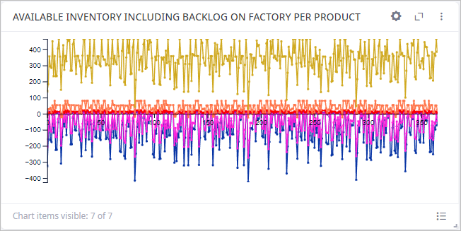
We can observe an Available Inventory page of results. In the second graph (Available Inventory Including Backlog on Factory per Product) we can see that availability of certain products in factory is dropping below 0, but it does not affect the service level. That decrease in available inventory is conditioned by the fact that body and metal frame have Order on demand policy. When an order is made, but no inventory is on hand, the amount is backlogged, and this is considered a negative value on a chart.

Now, since we analyzed both scenarios separately, we can get to the final step — compare two scenarios.

Both scenarios should be imported to run the Comparison experiment.

To see the Comparison experiment settings, we need to open Comparison experiment tile in either of the scenarios. We can add different statistics to this experiment from the pool of available statistics in the Statistics Configuration control. We have predefined certain statistics on the dashboard.

The first page of the experiment results contains all the selected statistics.

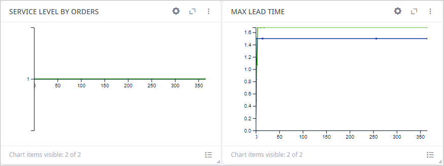
As we can see the Service Level by Orders is the same for both scenarios, and it is the maximum available value. the Max Lead Time is lower in the baseline scenario, which is better, because there is more time available for dealing with unpredicted, urgent situations before delivery becomes longer than the Expected Lead Time.

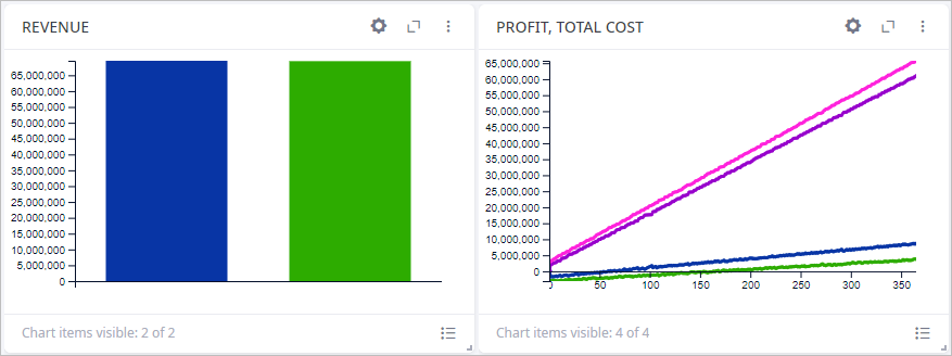
Revenue is almost the same, this little difference is only of stochastic nature, because demand is the same in both scenarios. Which means that the difference in profit is only due to difference in Total Cost.

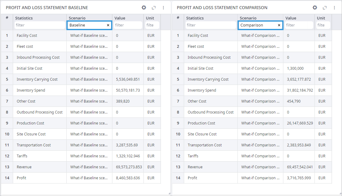
The Profit & Loss comparison page contains comparison of the Profit and loss statement tables. To make statistics more convenient for analysis we need to will filter the Scenario column of each table by the scenario name.

• In the first table type baseline in the filter field of the Scenario column.
• In the second table type comparison in the filter field of the Scenario column.

Eventually the table should look like this:

Now we can analyze these tables.

• First difference in values we see is the Initial Site Cost which is in the company's own production scenario due to necessity of opening new facilities. In the baseline scenario Initial Site Cost is 0, because supply chain is already working and there is no need to add new sites.
• The Inventory Carrying Cost is larger in the baseline scenario because there should be more products in storage. From China the products can be delivered only once in 14 days, so to maintain the same demand the company should order products in big batches.
• The Inventory Spend is much smaller in the comparison scenario because in this case the company orders only components and raw materials instead of buying finished products.
• Other Cost have insignificant difference.
• Production Cost is present only in the comparison scenario because only in this scenario toasters are produced by the company and not bought from the supplier.
• The tariffs in opposite is relevant only for the baseline scenario, because they are applicable only if product enters the EU. There are no tariffs for transferring products between countries inside the EU.
• Transportation Cost is larger for the baseline scenario simply because products should be delivered to the EU by the container ships.

There are different advantages and disadvantages in both scenarios, but the baseline supply chain is more profitable than the new one, and the gap in profit is only increasing as the time goes. That is why decision should be made to stick to the old strategy and continue to order toasters from the China supplier.

How can we improve this article?

Send