In the previous phase we imported scenario with optimized data, added suppliers, which will be servicing our distribution centers, created and configured inventory and sourcing policies.

In this phase we will configure and run Simulation experiment.

Open Simulation experiment's parameters

1. In the experiments section click the Simulation experiment tile to open its controls.

   

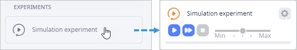
2. In the expanded tile click the Show settings icon to open the experiment's settings.

   

We will define the parameters of the experiment now.

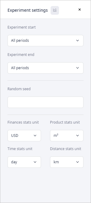
Define Simulation experiment parameters

1. Click the Product stats unit drop-down list and select pcs to define the measurement unit to be used in the statistics.

   Proceed to specify statistics that must be collected during the Simulation experiment.

2. Click the Statistics configuration icon to open the Statistics configuration dashboard below the map, which allows you to select and configure the required statistics.
3. By default almost all statistics are enabled. We will disable all statistics to further enable only the ones we need (Total Cost, Available Inventory and Demand Received (Dropped Orders)).
   • Click Enable All. Now all statistics are enabled, and the button is substituted with Disable All.
   • Click Disable All to disable all statistics.

   Now that all the statistics are unchecked, you may either scroll down the whole list of all the available statistics to check the ones we will use during the experiment, or you may filter them by their names.

4. Type Total Cost in the search field. The statistics will be automatically filtered. You will see the Total Cost statistics of Finances value type.

   

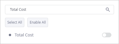
5. Click the toggle box to the right of it to activate data collection for the current statistics.
6. In the same way enable the Available Inventory and Demand Received (Dropped Orders) statistics.
7. Once you are done with configuring statistics, click the Statistics configuration icon to close the dashboard.
8. Now click Run on the experiment's tile.

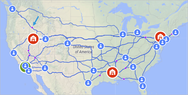
   The GIS map will appear allowing us to observe the real-time simulation (current model time considering the experiment speed) of the supply chain with shipments (purple dots) shipped from distribution centers to the customers and from the supplier to the distribution centers.

   

Our next step is to add the statistics that we want to compare. It can be done in the dashboard, which is located in the lower part of the anyLogistix workspace. The dashboard is divided into two areas:

• The section on the left is displaying the list of available dashboard pages. You can switch between pages, add new pages and remove the existing pages.
• The contents section on the right is displaying the contents of the currently selected page. The Dashboard page is selected by default (you can rename it if needed by right-clicking and selecting Rename from the pop-up menu).

Add statistics to the dashboard

1. Click the + Add New Chart button to open the chart settings dialog box.
2. In the dialog box click the + Add statistics drop-down list.
3. Select the checkbox next to the Total Cost statistics.

   

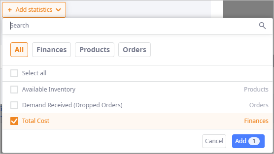
4. Click Add to add the statistics to the dashboard element.
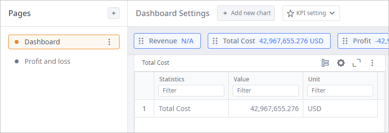
5. Click Apply. The Total Cost statistics will appear on the dashboard in the form of a table showing the total costs for the current moment.

   

Now we will add Available Inventory and Demand Received (Dropped Orders) statistics to the dashboard:

Add new statistics to the dashboard

1. Click the + Add New Chart button.
2. In the dialog box click the + Add statistics drop-down list.
3. Select the checkbox next to the Available Inventory statistics.

   

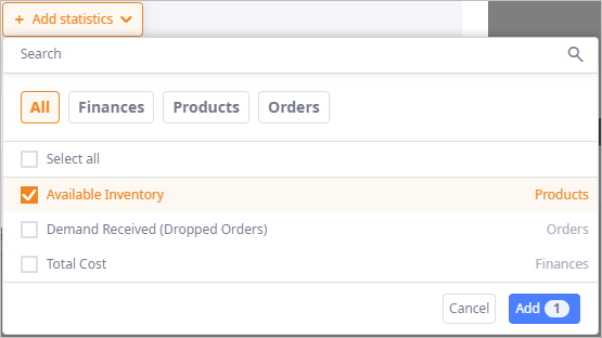
4. Click Add to add the statistics to the dashboard element.
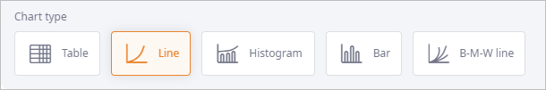
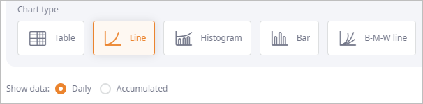
5. Set Line as its Chart type.

   

6. Click Apply to close the dialog box. The selected statistic will appear on the dashboard in the form of a Line chart to the right of the previously added Total Cost statistics.

   

7. In the very same way add the Demand Received (Dropped Orders) statistics to the dashboard:
   • Leave its chart type set to Table.
   • In the statistics parameters section select the Per Item toggle button referring to the Object parameter, allowing us in such a way to monitor statistics per object, i.e., we will see the quantity of orders lost at every warehouse.
     The Preview section will show the updated table view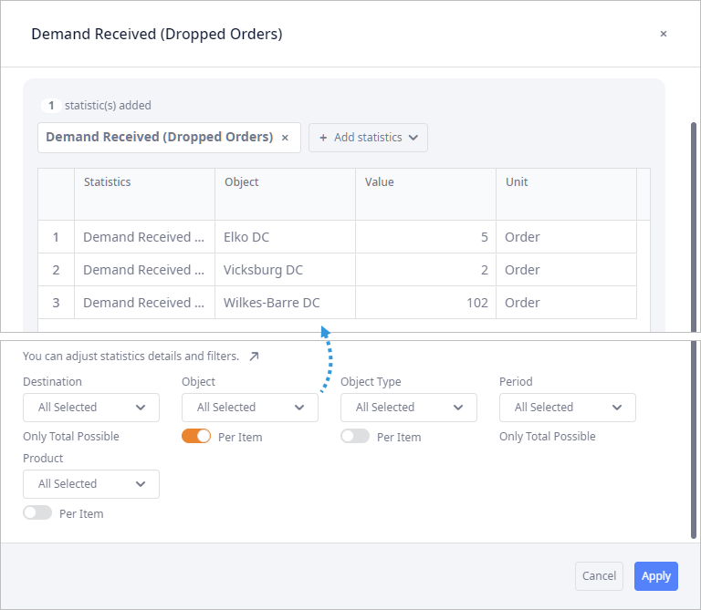

     

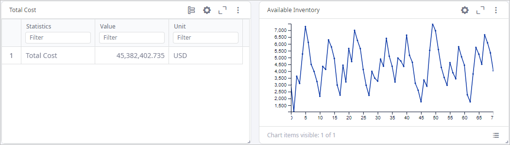
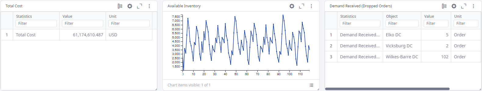
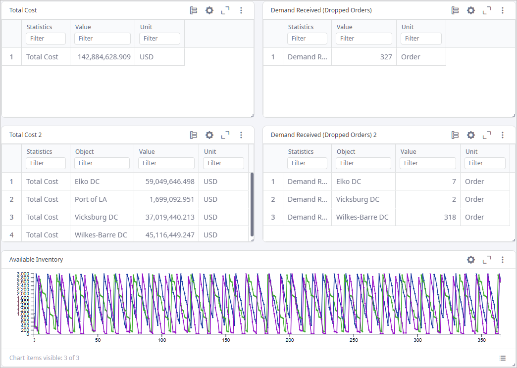
8. Click Apply to close the dialog box. The dashboard will now show the total cost statistics, the available inventory level (as well as the way it changes over time) and the quantity of lost orders per site.

   On the screenshot below you can see the three statistics that we intended to monitor, with the Demand Received (Dropped Orders) statistics providing data on each DC individually.

   Elements added to the dashboard can be rearranged to optimize occupied space.

   

Take a moment to monitor the collected Available Inventory statistics. You will see that the inventory level increases every time a new shipment from the supplier is received.

Have a closer look at the statistics

1. Click the Enlarge icon in the top-right corner of the Available Inventory chart.

   

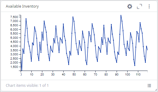
   The chart will be enlarged and placed over the anyLogistix layout.

   

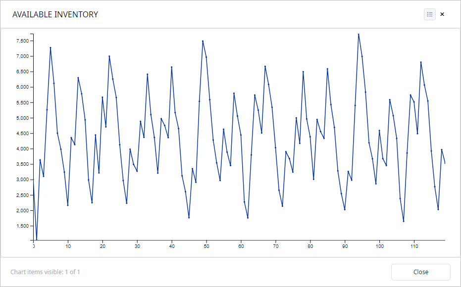
2. To get back to the compact view, click Close.

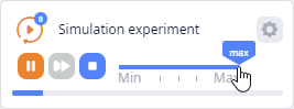
Let us increase the simulation speed and complete the experiment.

Increase the speed of the experiment

1. On the experiment's tile dtag the slider of the speed control to the right to set the speed to x2 value, which will correspond to two model days per second.

   

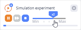
2. Then drag it to the max value. The experiment will be executed much faster and as a result it will be completed in a few seconds.

   

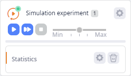
   When simulation completes, the result will be available in the Statistics item.

   

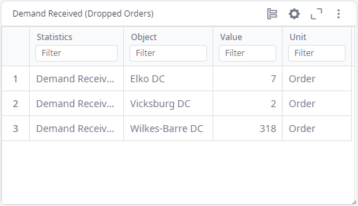
3. Now, if we look at the Demand Received (Dropped Orders) statistics we will see that 16 orders were lost at Elko DC, 2 orders were lost at Vicksburg DC and 323 orders were lost at Wilkes-Barre DC. We will have to modify the inventory policy later to eliminate the losses and to fully satisfy the demand.

   

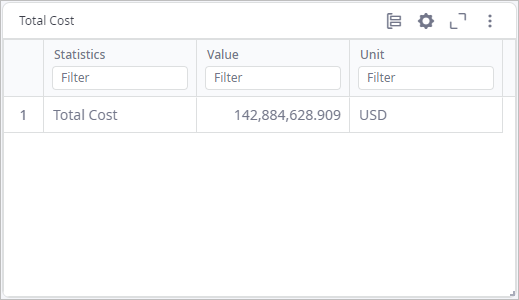
4. Lastly, let us take a look at the Total Cost table showing the expenses for all of the distribution centers. As you can see, it constitutes $142,127,302.917.

   

Alongside the total aggregated cost, we can examine the expenses incurred by each warehouse individually. This can be set in the settings of the dashboard element.

Examine statistics per item

To examine Available Inventory per warehouse, modify the element's parameters:

1. Click the cogwheel icon to modify the element's parameters. The chart's settings will open.
2. Define the parameter of the details and filters section to monitor statistics per object.
3. Click Apply to close the dialog box.

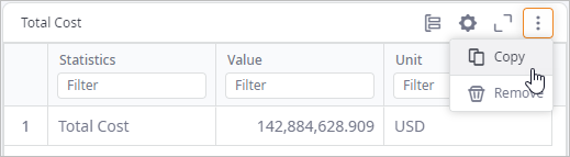
To examine Total Cost per item on a new dashboard element:

1. Click Copy on the Total Cost element and configure it to show data per object.

   

2. Click Apply to close the dialog box and add the statistics onto the dashboard.

   As compared to configuring the existing element, adding a new element allows you to have two independent dashboard elements offering aggregated total cost of all the objects and total cost per each individual object. We suggest that you should add a new element.

Before we proceed, we will add one more Demand Received (Dropped Orders) element showing the total amount of dropped orders for all warehouses.

Add new Demand Received (Dropped Orders) element

1. Click Copy on the Demand Received (Dropped Orders) element and configure it:
   • Chart type: Table
   • Disable the Per item toggle button of the Object parameter.
2. Click Apply to close the dialog box and add the statistics onto the dashboard.

Now we can see the results of our simulation experiment in details.

The results clearly show that we have lost certain amount of orders. The orders are dropped primarily because of the Backorder Policy (defined in the Demand table), which is set to Not allowed.

Let us analyze the data on dropped orders and find the moment the first order was lost.

Analyze Demand Received (Dropped Orders) statistics

1. Adjust the settings of the Demand Received (Dropped Orders) statistics that show data per object.
   • Click the cogwheel icon.
   • Set Line as the chart type for the current statistics.
   • Select the Daily radio button to observe data received per day, rather than the sum of the collected data.

     

   • Click Apply to save the changes and close the dialog box.
2. Click the Enlarge icon.
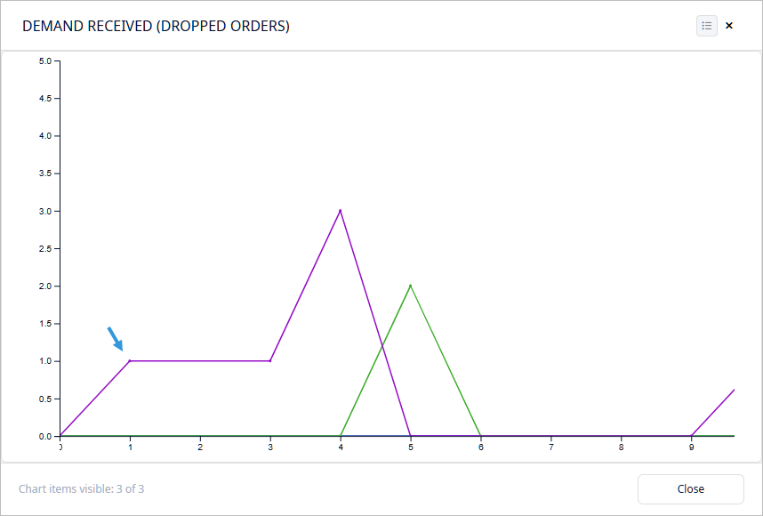
3. Left-click at the beginning of the chart and drag the mouse to the right to select the horizontal range containing the data on the first lost orders.

   

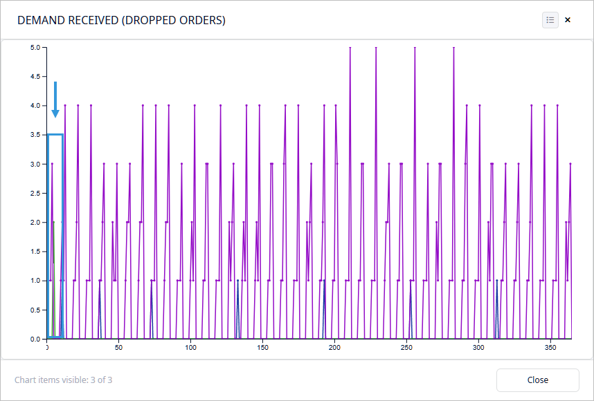
   You will zoom in to the selected range. As you can see, 2 orders were lost on the 4th day, which means that the initial amount was not sufficient.

   

You can run a number of what-if scenarios, adjusting the inventory policy parameters and examining the difference among the numerous received results.

Run what-if scenarios

1. Navigate to the Inventory table.
2. Open the pop-up dialog box by double-clicking the Policy parameters cell in the DCs row.
3. Adjust the Min and Max values by typing in the 3000 and 5000 respectively.
4. Set the Initial Stock, units to 1500.
5. Navigate back to the Simulation experiment and run it.
6. Voila — we have lost no orders, but as you can see, the expenses have increased as well and now constitute $172,138,904.816

We have successfully completed the Simulation experiment.

During this tutorial we learned to configure inventory policies, improved service level by eliminating the possibility of lost orders and executed what-if scenarios to find the optimal product stock volume.

To completely avoid losing orders, save your time on what-if scenarios, minimize the expenses and find the best possible inventory level — you should use the Variation experiment.

How can we improve this article?

Send